Learn spatial SQL and master GeoPackage with QGIS
For some reason, tutorials related to spatial SQL seem to focus on finding and analyzing the locations of bars. This tutorial goes in the line and helps the learners in analyzing those datasets on bars in their preferred locations with some spatial SQL in QGIS. QGIS is a great tool for this!
So, what we want to do is calculate the number of bars per neighborhood in the city of Leon, Mexico. With quite a few service points (INEGI: dataset on services DENUE) and big set of neighborhoods (Iplaneg) in the whole state of Guanajuato (where Leon is located), the best way to resolve this puzzle was with spatial SQL. It’s to say with a query based on Structured Query Language (SQL), that would serve us in building a code-based, reproducible and transparent (ie. readable) workflow towards analyzing our spatial data.
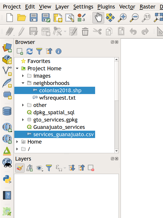
Data formats matter. With Geopackage we have the possibility to work with our data in a file-based database environment that supports SQL with a variety of spatial functions. Let’s take the data in then. In QGIS it happens basically by drag and drop, and that’s it: you’ll get rid of those shapefiles.
The neighborhoods data (colonias2018.shp) was converted to GeoPackage format by ‘drag and drop’ using the Layers- and Browser-panels in QGIS, whereas the data on services was originally in .csv-format. I had it imported to QGIS and then exported (Save Vector Layer as…) with a CRS-conversion to our GeoPackage-file.

As GeoPackage is a database, we need to understand the layers in it as tables that have just a set of rows and columns like a spreadsheet. Usually, each row or record of a table contains information about geometry just like the “attribute tables” with the traditional geospatial data formats like shapefiles. What’s the difference then? The information on geometries is stored in a column and all the data is stored very efficiently making your work faster.
Before starting with those powerful SQL queries we just need to ensure that our GeoPackage layers are indexed. The indexes are hugely important for the databases; index makes the database to work the data in an ordered matter and makes your analysis a lot faster.
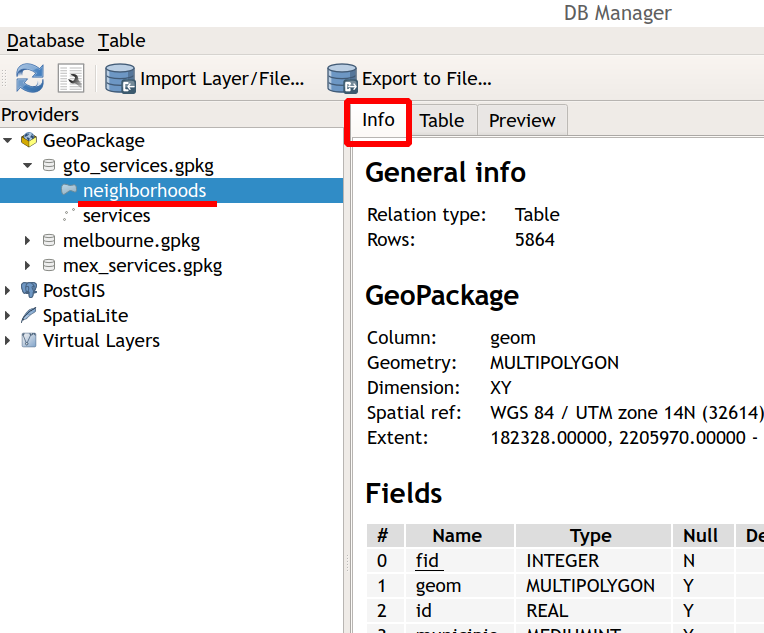
Next we open the DB Manager in QGIS and preview the info for the data layers. Scrolling down we’ll see that there are no indexes just yet. To create the indexes we should open from the upper menu “Table” and the “edit table” option.
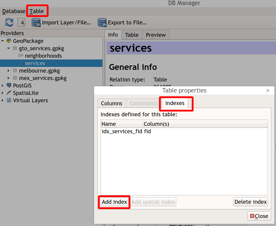
Now we can add indexes and we should do this layer by layer.
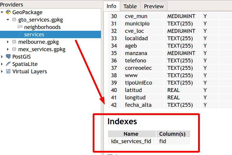
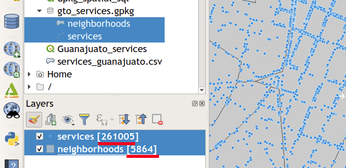
Now we can browse our data and see how many features we will work actually. Above, we can see the data in action, as we can see that, especially, the services table is quite numerous.
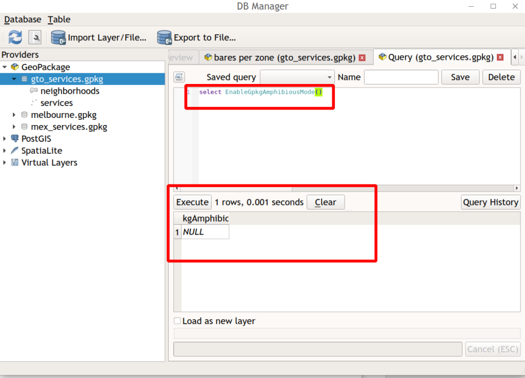
Then we’re off to make those SQL queries. First, we have to pass along a somewhat strange-looking command to the SQL query editor of the DB manager :
select EnableGpkgAmphibiousMode()
This enables QGIS to work optimally with Geopackage spatial functions and makes “SpatiaLite to work natively with GeoPackage geometry, removing the need to explicitly call the appropriate format conversion functions such as GeomFromGPB() or CastAutomagic()”, as Bryan McBride from Spatial Networks defines it in the company blog on the subject.
We can start with some basic queries and move towards our initial goal, to quantify the bars in the different neighborhoods of León.
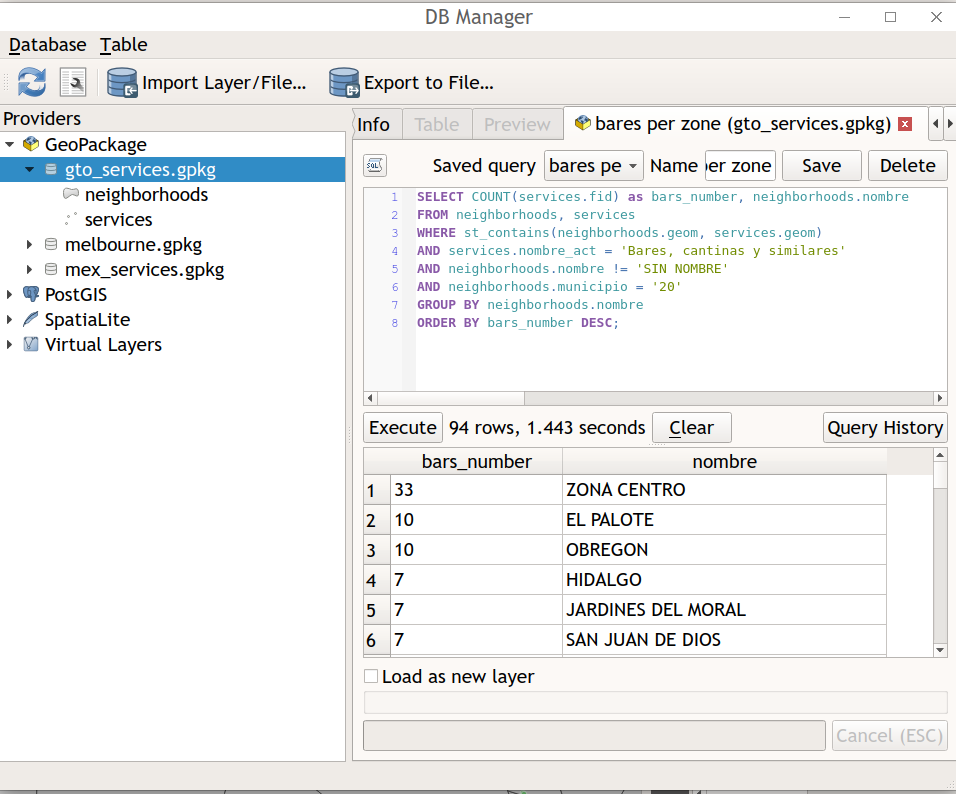
As we can see besides Execute button, 1.443 seconds is quite fast, right? Imagine leaving behind those multi-step button clicking GIS processes and moving towards the utilization of commands to produce effective and reproducible GIS workflows of minimum length in time.
So, what did we actually do? We did a query on the data. As we can recall, a query is a request for data from a database table or combination of tables.
SELECT COUNT(services.fid) as bars_number, neighborhoods.nombre
FROM neighborhoods, services
WHERE st_contains(neighborhoods.geom, services.geom)
AND services.nombre_act = ‘Bares, cantinas y similares’
AND neighborhoods.nombre != ‘SIN NOMBRE’
AND neighborhoods.municipio = ‘20’
GROUP BY neighborhoods.nombre
ORDER BY bars_number DESC;
Don’t let the Spanish words fool you! It ain’t that hard!
— first, we’ll use the count-function to help us counting the requested data
SELECT COUNT(services.fid) as bars_number, neighborhoods.nombre
— then we’ll define the tables
FROM neighborhoods, services
— and the where-clauses that include the spatial intersection between the two tables
WHERE st_contains(neighborhoods.geom, services.geom)
AND services.nombre_act = ‘Bares, cantinas y similares’
AND neighborhoods.nombre != ‘SIN NOMBRE’
AND neighborhoods.municipio = ‘20’
— and here we’ll group the requested data by the neighborhood
GROUP BY neighborhoods.nombre
— besides of ordering the results in a descending order
ORDER BY bars_number DESC;
Nice! Finally, we’re glad to point out to you that QGIS is moving rapidly towards using GeoPackage as the number one file-based spatial data format. Besides, it’s important to remark how well databases fit the future workflows of GIS data analyst or GIS technician: the datasets are getting bigger and there’s just no room and time to use inefficient data formats and archaic GIS workflows.
And if we’ll talk about next steps, say no more: PostGIS handled this query approximately 18 times faster.

As we can appreciate QGIS as a modern GIS platform that’s integrated with the best spatial algorithms and the most appropriate data formats to you to process your data in no-time. The part that falls behind in this equation is knowledge for understanding and utilizing geospatial data. This is why we at Gispo want to share with you the possibility to level-up your geospatial knowledge and software know-how in our online learning platform for open source geospatial knowledge building.
If you’re interested in the use of GeoPackage to gain productivity for your GIS processes, you’ll probably be interested also in learning how to do your other GIS tasks with the latest version of QGIS. If that’s the case, send us an e-mail at info@gispo.fi
